Breaking down GPT-2 and Transformer
GPT-2 has shown an impressive capacity of getting around a wide range of NLP tasks. In this article, I will break down the inner workings of this versatile model, illustrating the architecture of GPT-2 and its essential component — transformer. This article distills the content of Jay Alammar’s inspirational blog The illustrated GPT-2, I highly appreciate his awesome job of illustrating this game-changer model and recommend you to chew his insights directly if having any confusion as reading this digest.
What is GPT-2?
GPT-2 is a large-scale transformer-based language model that was trained upon a massive dataset. The language model stands for a type of machine learning model that is able to predict the next word given a sequence of word input. GPT-2, like other language models, output one word each time, which we called auto-regressive (BERT, instead, is able to incorporate both sides of context to gain better result, thus is not auto-regressive). At the core of GPT-2 is a stack of transformer decoders, each of which has the same architecture as below:

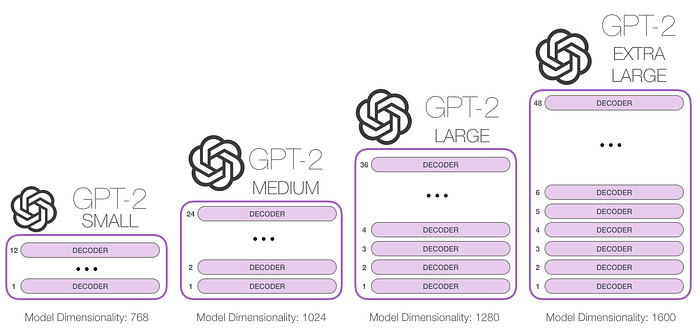
GPT-2 offers different choices of the model size (124M, 774M, etc) which are mainly distinguished by the number of transformer decoders stacked inside the model:
Here let’s first peek at the overall process of how GPT-2 predicts the next word at one step:
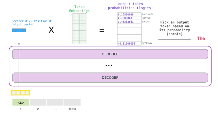
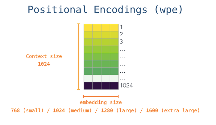
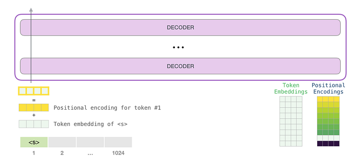
The above figure shows the first auto-regressive step of using GPT-2 to generate a sentence freely from scratch (which is technically called generating unconditional samples). <s> is the start token we usually pass into the model in this case. It is noted that to make the model able to process the input token, we have to convert the text token into a vector embedding beforehand (the yellow vector). In GPT-2, an input embedding of a token is the sum of token embedding and the corresponding positional embedding. Those two embeddings can be retrieved from pre-trained embedding matrices:

Without rolling out the details of intermediate transformers, the output of each path is an output vector with which we can calculate how likely each word in the vocabulary is to be the predicted token at this position (Figure 2). Usually, to ensure the output diversity, we will sample a word from top-k words. When top-k = 1, the model becomes deterministic which means that the output will not change across multiple running if the input is the same.
Self-attention mechanism
Let’s look back to the inner architecture of each decoder block (Figure 1). What jumps into our eye at first glance is the masked self-attention layer. So what is it for? In a nutshell, the self-attention layer is used to interpret and encode a word within its context. For example, to understand what “it” refers to in the following sentence:
Second Law of Robotics
A robot must obey the orders given it by human beings except where such orders would conflict with the First Law.
The model has to scrutinize the whole sentence so as to infer that “it” refers to “robot”.
Compared with traditional self-attention, masked self-attention only allows model to take care of the context to the left. Specifically, what a masked-attention layer does is to assign a score to each word in the window of context which represents how relevant the word is to the input one.
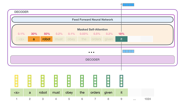
But how do we calculate this relevance score? In a transformer, there are three significant vectors that each input word has:
Query: The query is a representation of the current word used to score against all the other words (using their keys). We only care about the query of the token we’re currently processing.
Key: Key vectors are like labels for all the words in the segment. They’re what we match against in our search for relevant words.
Value: Value vectors are actual word representations, once we’ve scored how relevant each word is, these are the values we add up to represent the current word.
One analogy that Jay makes to illustrate the process of self-attention is sticky note matching. Imagine we have a note saying what word we are looking up (query vector), each folder is tagged with a label for matching (key vector) and has content value (value vector). Self-attention is going to use this query vector to score against the label of each folder (dot product following with softmax) and calculate the weighted blend of value vectors with these probabilistic scores.

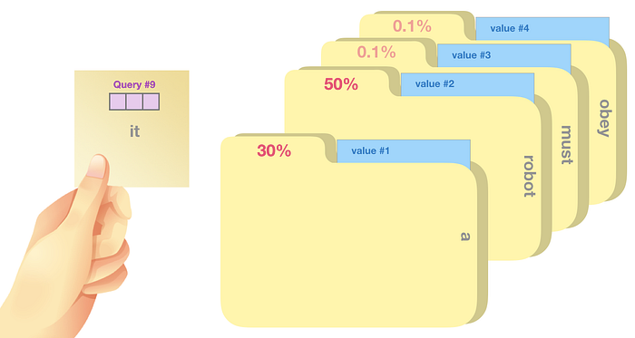
The process of calculating the output of the self-attention layer with “it” is like:
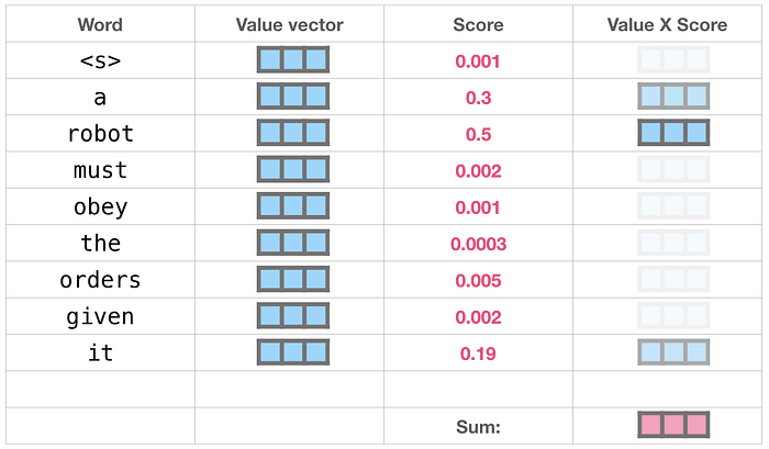
This weighted vector will be further fed to the next feed-forward neural network which projects the dimension of the self-attention output to that of input of the next transformer decoder block (Figure 2, since GPT-2 doesn't use transformer encoder, the second layer of the transformer in Figure 2 is discarded).
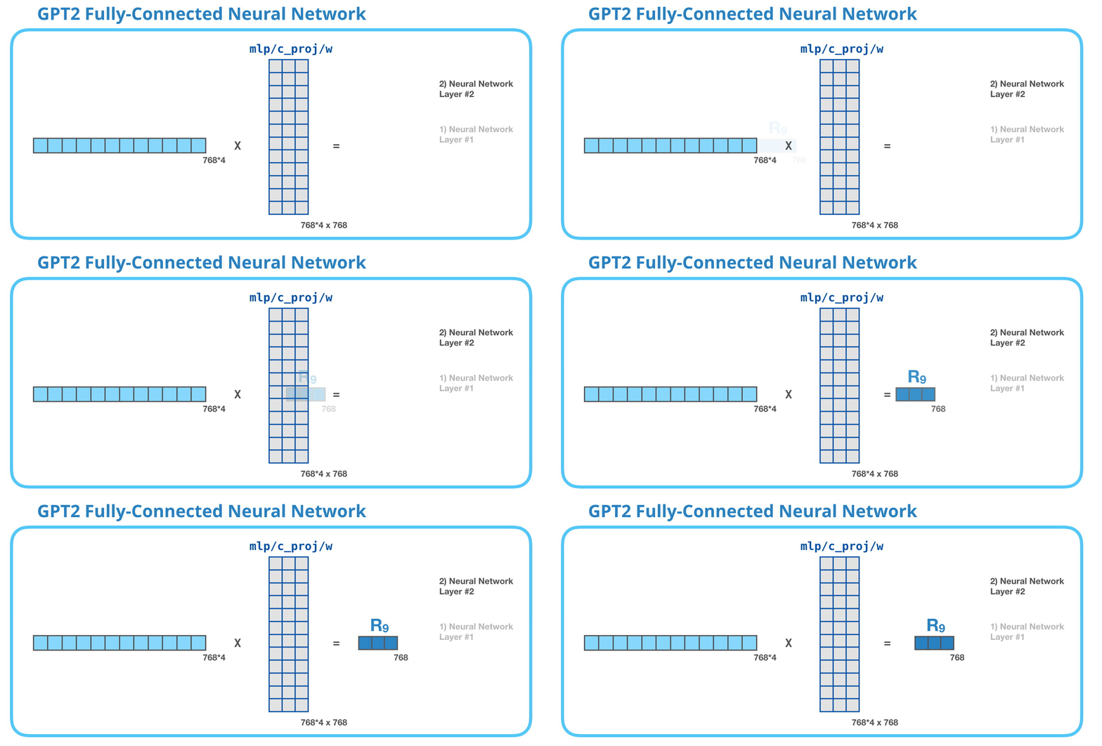
This feed-forward neural network consists of two layers: the output dimension of the first layer is four times of the model size (e.g. if mode size is 768, the output of the first layer should be 768*4), it may because that such configuration could give transformer enough representational capacity:
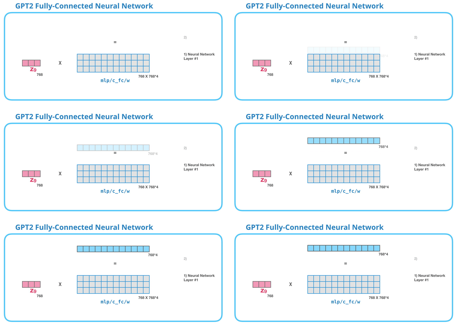
The second layer is to project the dimension of the first layer back to model size (which is also the dimension of transformer input).
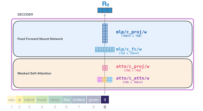
As a whole, the weight matrices that input vector encounters inside the transformer includes:
The last concept we haven’t tackled is “multiple attention heads”. In this case, each attention head maintains a set of Q, K, V vectors on their own. Getting the vector of each head can be easily implemented by reshaping the long vector into a matrix:
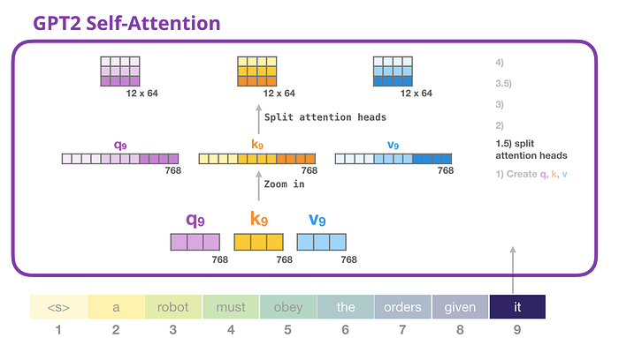
After reshaping, row i represents the vector corresponding to head i.
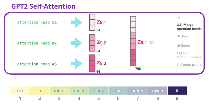
At the end of the self-attention layer, we will concatenate the output of attention heads into one long vector:
Enjoying the landscape of the whole GPT-2 model
Bravo! We finally flesh out the skeleton of GPT-2, let’s enjoy this masterpiece landscape!

Reference
The Illustrated GPT-2 (Visualizing Transformer Language Models http://jalammar.github.io/illustrated-gpt2/
Examining the Transformer Architecture https://towardsdatascience.com/examining-the-transformer-architecture-part-1-the-openai-gpt-2-controversy-feceda4363bb